
This page includes 10 popular graphical area displays that are used for weather analysis and forecasting. 1. GRAPHICAL AREA DISPLAY: CAPE CAPE stands for Convective Available Potential Energy. It can be thought of as the energy that is available for an updraft in a storm to rise. Generally, as CAPE increases then the storm updraft will increase and a storm will be more likely to have severe characteristics such as large hail, intense lightning and strong winds. CAPE is displayed on a Skew-T diagram. One limitation is that this CAPE value is only for one point location. Forecasters also look at CAPE displayed on a graphical area display to see how CAPE varies across a region. Another dimension can also be added by putting to the image into a time motion to see how CAPE varies over time. The map below shows an example of CAPE contoured over an area. Much of the region has CAPE values of 1,500 Joules/kg or higher. The guide below can be used to get a sense for how significant a CAPE value is when looking at these values: 1 to 1,500: Positive 1,500 to 2,500: Large 2,500+: Very Large 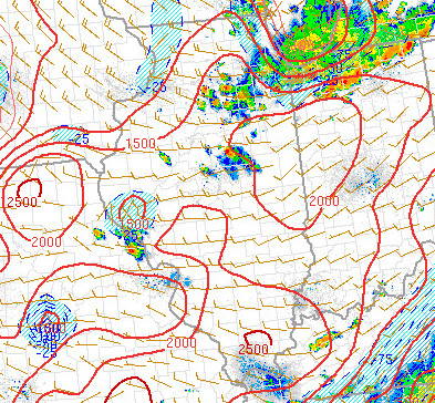 2. GRAPHICAL AREA DISPLAY: CAPE CHANGE CAPE (Convective Available Potential Energy) change shows how much the CAPE has changed over a given time period. A common time frame is the change over a 3 hour period. CAPE (when it is present) will tend to increase during the morning and afternoon and decrease in the evening and at night. Other considerations though can cause an increase or decrease in CAPE at different portions of the day compared to what typically occurs. Below are factors that can cause the CAPE to increase or decrease. It is a good idea to be aware of the factors that are causing CAPE to increase since it can contribute to stronger storms. There are also many factors that can cause CAPE to decrease. Factors that can increase CAPE 1. Increasing boundary layer temperature from solar radiation 2. Increasing boundary layer dewpoint from moisture advection 3. Low level warm air advection (warmer air moving into area) 4. Cooling aloft such as at 700 mb and 500 mb from cold air advection 5. A combination of 2 or more of the above Factors that can decrease CAPE 1. Decreased boundary layer temperature from the decrease or loss of solar radiation 2. Decreasing boundary layer dewpoint 3. Low level cold air advection 4. Warming aloft such as at 700 mb and 500 mb 5. Cooling from thunderstorm outflow 6. Increased cloud cover, especially overcast conditions 7. A combination of 2 or more of the above The image below shows an example of a 3 hour change in CAPE. In the example the CAPE has decreased. The larger the number, then the more significant the decrease. 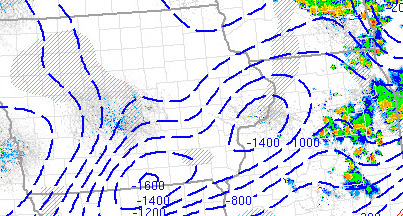 3. GRAPHICAL AREA DISPLAY: MU (MOST UNSTABLE) CAPE Instability may be present by lifting air from the surface and throughout the troposphere. The amount of instability present through this process is known as CAPE (Convective Available Potential Energy). This CAPE region is also known as positive area and it is where the theoretical rising parcel of air is warmer than the surrounding environmental air. Being warmer means it is also less dense and will rise freely like a helium balloon due to positive buoyancy. Lifting though does NOT have to be just initiated from the surface. The lifting can begin at any level within the lower troposphere. Because lifting can occur at a variety of different pressure levels, the amount of CAPE that is actualized for a given situation will depend on where the lifting starts from. Meteorologists have developed strategies to deal with this problem in order to get a better sense of how much instability or CAPE will be realized in a given atmospheric set-up. One of these is called Most Unstable CAPE. To get this value, first it is determined how much CAPE is present when air is lifted from a variety of different pressure levels between the surface and about 700 millibars. For example, one parcel will be lifted from the surface, another from 975 mb, another from 950 mb, etc. Each of these situations will have a unique CAPE and these CAPES will vary in magnitudes. The Most Unstable CAPE picks the highest of these values. The image below shows an example of Most Unstable CAPE. Very high instability values exist over Oklahoma and Arkansas on this example. 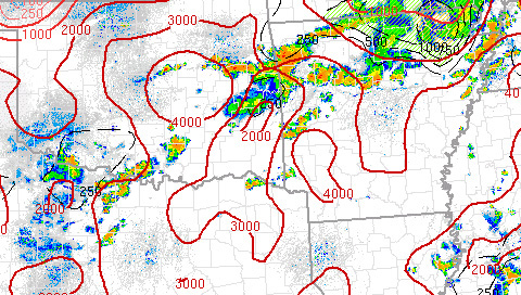 4. GRAPHICAL AREA DISPLAY: DD (DOWN DRAFT) CAPE The down draft is the air that rushes out of a thunderstorm and to the ground. Once it gets the ground, it fans out in all directions similar to a water balloon breaking when hitting the ground. These down drafts are what are responsible for causing convective wind gusts. Another term used is �straight line wind� in order to discern it from the rotational winds of a tornado. Just like tornadoes, straight line wind can have a variety of different wind speeds although straight line wind generally has a weaker wind than a moderate or strong tornado. Straight line wind is severe when the wind speed exceeds 50 knots (58 mph). These speeds can cause damage to fencing, houses and objects vulnerable to the wind. Down Draft CAPE is an index that helps give the forecaster an idea of how strong convective wind gusts will be. Several of the actual physical variables that help produce a stronger down draft include: 1) a higher CAPE (more instability) 2) dry air in mid-levels (~700 to ~500 mb) (evaporative cooling supports negative buoyancy which causes the air to sink faster to the surface 3) supercell storm or linear band of severe storms (energy is focused into one region or along a single axis allowing for plenty of potential energy to be converted into storm kinetic energy) 4) Warm air in the boundary layer (the contrast in air density between the heavy colder air and lighter warm air will allow for a more intense down draft The image below shows an example of down draft CAPE. The higher the value then the greater the potential for a stronger downdraft. There can be significant errors in the values of down draft CAPE due to spatial resolution of actual observations and contamination from air mixing in the boundary layer but it gives the forecaster a general idea if stronger down drafts can be expected. Values below 600 and especially closer to zero are associated with weaker down drafts and values over 1,000 and especially over 1,500 are associated with very strong down drafts. This is a generality since any storm is capable of producing severe convective wind gusts given the right set of conditions. 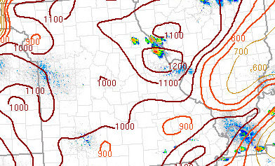 5. GRAPHICAL AREA DISPLAY: LI (LIFTED INDEX) Like CAPE, LI (Lifted Index) assesses instability. It compares the actual 500 mb temperature to the theoretical temperature at 500 mb that would result from a parcel of air rising from the boundary layer to 500 mb. If the parcel temperature is warmer than the actual 500 mb temperature then the LI is negative. A negative LI indicates instability and the more negative the value then the more unstable the air. Unlike a single Skew-T sounding, a map can show how the LI varies over a big area. Multiple sounding stations, various model runs and current weather data can be used to calculate the LI over an entire region. The example below shows Lifted Index over Illinois and nearby areas. The LI values are very negative and this indicates strong instability. Storms developing in this region from surface based convection can be expected to have very strong updrafts. This increases the likelihood for severe weather such as severe convective wind gusts and large hail. Notice the stabilizing influence over Lake Michigan. This results because the water heats up less than the land. The warmer temperatures over the land lead to higher values of instability. LIFTED INDEX Positive number: Stable 0 to -4: Marginal instability -4 to -7: Large instability -8 or less: Extreme instability 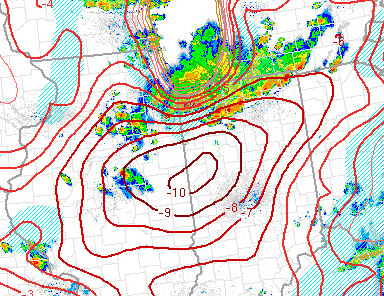 6. GRAPHICAL AREA DISPLAY: 850 to 500 mb LAPSE RATE A lapse rate is a change in temperature with height. This value can be used to infer instability. The higher the value then the higher the instability. Values less than 6 are generally stable while values of 7.5 or above are very unstable. Values between 6 and 7.5 generally mean there is instability and it can be released if there is adequate dynamic lifting to lift a parcel into an unstable elevation in the troposphere. The same holds for values of 7.5 and above, but the convection is more likely to be explosive if instability release occurs at these high values. The 850 and 500 mb lapse rate has units of �C/km�. The �C� value is found by taking the temperature difference between 850 and 500 mb. The �km� value is the vertical distance between the 850 and 500 mb pressure surfaces. For example, if the temperature is 25 C at 850 mb, the temperature is -10 C at 500 mb, and the distance from 850 to 500 mb is 4.2 km, then the lapse rate is (25 �(-10) / 4.2 = 35/4.2 = �8.3 C/km�. For higher elevation regions, such as locations where the 850 mb level is near or below the ground surface, then the 700 to 500 mb lapse rate is used in order to represent the lapse rate. The image below shows an example of a lapse rate chart. The values are on the high side, thus thunderstorms that develop should have strong updrafts. This increases the potential for severe weather. 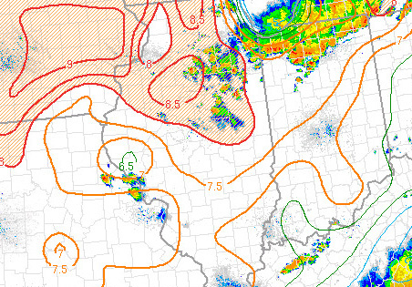 7. GRAPHICAL AREA DISPLAY: K INDEX The KI is a combination of the Vertical Totals (VT) and lower tropospheric moisture characteristics. The VT is the temperature difference between 850 and 500 mb while the moisture parameters are the 850 mb dewpoint and 700 mb dewpoint depression. KI = (T850 - T500) + (Td850 - Tdd700) Operational interpretation of value obtained: 15-25: small convective potential 26-39: moderate convective potential 40+: high convective potential The image below shows an example of a map of K index values. Many of the values on the map are 30 or greater. This indicates a significant threat for convection. High values suggest there is enough moisture and instability to support thunderstorms if there is adequate lifting. The value can be misleading at times thus it is a good idea to check over a variety of weather data (CAPE, LI, surface dewpoints, wind shear, dynamic lifting mechanisms, capping, convective instability, etc.) to get a better feel for the convective potential and storm characteristics that storms could have if they develop (severity, tornadic potential, etc). 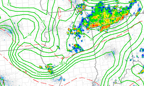 8. GRAPHICAL AREA DISPLAY: LCL (LIFTING CONDENSATION LEVEL) The LCL (Lifting Condensation Level) is the height in meters above the ground surface at which a rising parcel of air first becomes saturated. This level is found theoretically in several similar ways. A common way is to determine the average temperature and dewpoint between the ground surface and 50 mb above the ground surface. Use these temperature and dewpoint values for a parcel of air that is force lifted from the lower PBL (Planetary Boundary Layer: layer of air closest to ground surface where friction and thermal mixing is common). The elevation that this parcel of air first becomes saturated (relative humidity = 100%) is the LCL. One assumption that must be made is that the lifting is occurring from the lower PBL, thus the LCL is only relevant for lifting that is occurring from the PBL and not lifting that is starting higher aloft such as lifting that first starts above the PBL. Thus, the LCL is most relevant to warm season convection that is helped in the initiation process by solar warming of the ground surface in the PBL. LCL is not relevant for cool season convection that is initiated above the PBL or for any convection that first starts above the PBL. There are a couple of reasons why this value is important to operational meteorology. First, it gives an indication of how high cloud bases will be. If the PBL is moist (high relative humidity) then cloud bases (the bottom of clouds) will tend to be lower in elevation and thus closer to the ground surface when surface based convection occurs. A hot and dry PBL will lead to very high cloud bases and significant lifting will need to occur to lift the air high enough in order for saturation to occur. A LCL value of 1,500 m and especially less than 1,000 m is relatively close to the ground while a value greater than 2,000 m and especially greater than 3,000 m are relatively high. Second, An LCL closer to the surface (assuming the LFC (Level of Free Convection, which will be further analyzed in next writing) is relatively close to the surface also) indicates a greater potential for tornadic development. Of course, other factors such as wind shear and instability need to be significant and influencing the lower troposphere. With no other limiting factors, a LCL and LFC close to the ground surface will allow the region of CAPE and wind shear to be overlapped close to the ground surface. This makes it more likely a tornadic circulation can occur. The image below is an example of LCL height shown over an area. 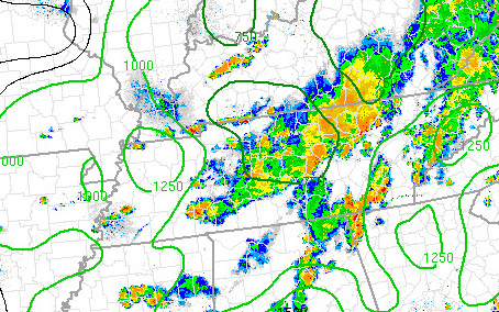 9. GRAPHICAL AREA DISPLAY: LFC (LEVEL OF FREE CONVECTION) The LFC (Level of Free Convection) is the height at which the region of instability begins when the CAPE profile is known. This marks the elevation at which a parcel of air will rise on its own due to positive buoyancy. The Level of Free Convection value will depend on several factors such as temperatures in the PBL, dewpoints in the PBL, and the temperature profile from the PBL to the middle levels of the troposphere. Contributors to instability are high PBL temperature, high PBL dewpoint and relatively cool air in the middle troposphere (i.e. 700 to 500 mb). When instability is present, the LFC marks the bottom of the region of instability. The LFC value is given in meters and this value indicates how high above the ground the region of instability begins. A low LFC value indicates the LFC is relatively close to the surface while a high LFC values indicates the LFC is relatively high above the surface. Values less than 1,000 meters are relatively close to the ground surface while values above 2,000 meters are relatively high above the ground surface. The Level of Free Convection is looked at in the context of a thunderstorm situation. If there is no instability, then there will be no LFC. Thus, surface based thunderstorms have to be possible before the LFC is relevant to study. If thunderstorms are expected, then the next step is to determine if those storms could be severe and what severe characteristics they will have. LFC is looked at when making a tornadic thunderstorm forecast. If no other limiting factors are present for tornadic thunderstorms, then a LFC relatively close to the surface will increase the tornadic threat. This is because there is better overlap between instability and wind shear in the lower troposphere. The image below is an example of how contours of LFC will look on a map. 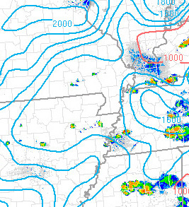 10. GRAPHICAL AREA DISPLAY: RH BETWEEN LCL and LFC When CAPE is present from the potential for surface based convection, the sounding profile will have both a LCL and a LFC. The LCL is the Lifting Condensation level. This is the height that a parcel first becomes saturated when force lifted from the lower PBL. The LFC is the Level of Free Convection. This marks the bottom of where the region of CAPE and instability first begins. The LFC will be at or above the LCL in elevation. The vertical distance between the LCL and the LFC will vary. The relative humidity between these two levels will also vary. Instability, thunderstorms and severe storms will have a greater magnitude or threat when the LCL and LFC are relatively close together and the relative humidity between these levels is relatively high. The reasons for this can include: CAPE starting closer to the surface, less entrainment of dry air into the updraft as it is force lifted from the LCL to the LFC, and better overlap between instability and wind shear in the lower troposphere given the presence of significant low level wind shear. The image below shows as example of an area display of relative humidity between the LCL and LFC in the black dashed lines. Values above 70% are relatively high while values below 60% are relatively low. If no other limiting factors are present, high LCL to LFC RH values will enhance instability and storm strength. 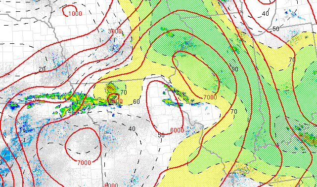 |